
Expectation-Maximization (EM) algorithm part I (Introduction)
Published:
Introduction
Maximum likelihood estimation (MLE) is a way of estimating the parameters of a statistic model given observation. It is conducted to find the parameters that maximize observations’ likelihood under certain model distribution assumptions. However, in many real life problems, we are dealing with problems with parameters that are not directly available to infer given the limited data we have, which are called hidden variables Z. Many problems in the areas of genomics involve dealing with hidden variables. Typical examples in genomics are (i) inferring microbial communities (Z: different communities) (ii) inferring the ancestries of a group of individuals (Z: different ancestries) (iii) inferring the cell type content from specific sequencing data (Z: different cell types). Problems involving hidden variables like these are typically hard to directly performing maximum likelihood estimation.
Motivating example
Using an application to motivate the abstract math formula is more intuitive to understand. So before going into any math detail, let’s use the popular 1000 Genome dataset as an example. In the example dataset, we have approximately 1000 individuals (n) from different ancestries; each individual has ~13k carefully selected SNPs (m). Formally, let’s denote it as X, which is a $ n \times m $ matrix with value ${0, 1}$, or the haplotype matrix. The objective is to learn, without being given explicitly, the ancestry of each individual in an unsupervised approach.
EM algorithm
Let’s assume we believe there are $K$ difference ancestries. Denote \(\pmb{X}_{i,j}\) as the genotype data of individual $i$ at SNP $j$. Let’s say the $j^{th}$ SNP in individual $i$ is passed by ancestry $k$, and ancestry group $k$ has $f_{k,j}$ chance to pass a value $1$ at SNP $j$ to the offspring. Let’s denote $\pmb{Z}$ as a ancestry matrix of each individual, so that $\pmb{Z}_{i,k} = 1$ means individual $i$ belongs to the ancestry group $k$. The prior distribution of $\pmb{Z}$ is determined a multivariate normal distribution characterized by $ \pmb{\pi} $. (If you wonder why we are making all these assumptions, please check my Li-Stephens HMM blog for more details). Mathematically:
\[\pmb{Z}_{i}|\pmb{\pi} \overset{iid}{\sim} Mult(\pmb{\pi}), \quad \pmb{X}_{i,j} | (\pmb{Z}_{i,k} = 1) \sim Ber(f_{j,k})\]Given we have the ancestry information matrix \(\pmb{Z}\), solving for parameter parameter $ f_{k,j} $ is easy:
\[P(\pmb{X}, \pmb{Z} \vert \pmb{f},\pmb{\pi}) = \prod_{i=1}^N \prod_{k=1}^K \pi_k P(\pmb{X}_i\vert \pmb{Z}_{i,k} = 1)^{\mathbb{1}\{\pmb{Z}_{i,k}=1\}}\]Where the last equation is based on the (simply, but usually unrealistic) assumption that each SNP is independent to each other. Then we can solve the above equation using Maximum Likelihood Estimation (MLE) easily. For simplicity, let’s use $\pmb{\theta}$ to be the parameters we want to learn above. To rewrite the above equation in log form, we have
\[\log(P(\pmb{X}, \pmb{Z} \| \pmb{\theta})) = \sum_{i=1}^n\sum_{k=1}^K \mathbb{1}\{\pmb{Z}_{i,k}=1\}\log(\pi_k p(\pmb{X}_i \| \pmb{f}_k))\]What makes it hard is when we do not observe the ancestry groups \(\mathbf{Z}\). Then we need to infer the probability of ancestry given the observation \(\mathbf{X}: P(\mathbf{Z} \vert \mathbf{X}, \mathbf{\theta})\). But this requres us to know \(\pmb{\theta}\) first! This comes to the first step of EM algorithm: initialize the parameters as \(\mathbf{\theta}^{(0)}\). After we cheat the posterior \(P(\mathbf{Z} \vert \mathbf{X}, \mathbf{\theta}^{(0)})\), we can form the complete data likelihood to learn the updated parameter \(\mathbf{\theta}\) :
\[\begin{align*} Q(\pmb{\theta}, \pmb{\theta}^{(0)}) &= E_Z [\log(p(\pmb{X}, \pmb{Z} \vert \theta))] \\ &= E_Z [\log(p(\pmb{Z})p(\pmb{X} \vert \pmb{Z}, \theta))] \\ &= \sum_{i=1}^n\sum_{k=1}^K P(z_k \vert x_{i}, \pmb{\theta}^{(0)}) \log(\pi_k \prod_{j=1}^m p(x_{i,j} \vert f_{j,k})) \end{align*}\]and the cheated posterior can be learned as
\[\begin{align*} &P(z_k | x_i, \pmb{\theta}^{(0)} ) =\frac{P(x_i| z_k, \pmb{\theta}^{(0)})P(z_k|\pmb{\theta}^{(0)})}{P(x_i| \pmb{\theta}^{(0)})} \\ & = \frac{\pi_k^{(0)} \prod_{j=1}^mf_{i,j}^{(0)x_{i,j}}(1-f_{i,j}^{(0)})^{1-x_{i,j}}}{\sum_{k=1}^K\pi_k^{(0)} \prod_{j=1}^mf_{i,j}^{(0)x_{i,j}}(1-f_{i,j}^{(0)})^{1-x_{i,j}}} \end{align*}\]This is called the Expectation step (E-step). After we learned the posterior, we plug it back to get the $Q(\pmb{\theta},\pmb{\theta}^{(0)})$ and find the parameters $\pmb{\theta}$ that maximize the function. (M-step). We perform the abovementioned step several times until converge.
Experimental Results
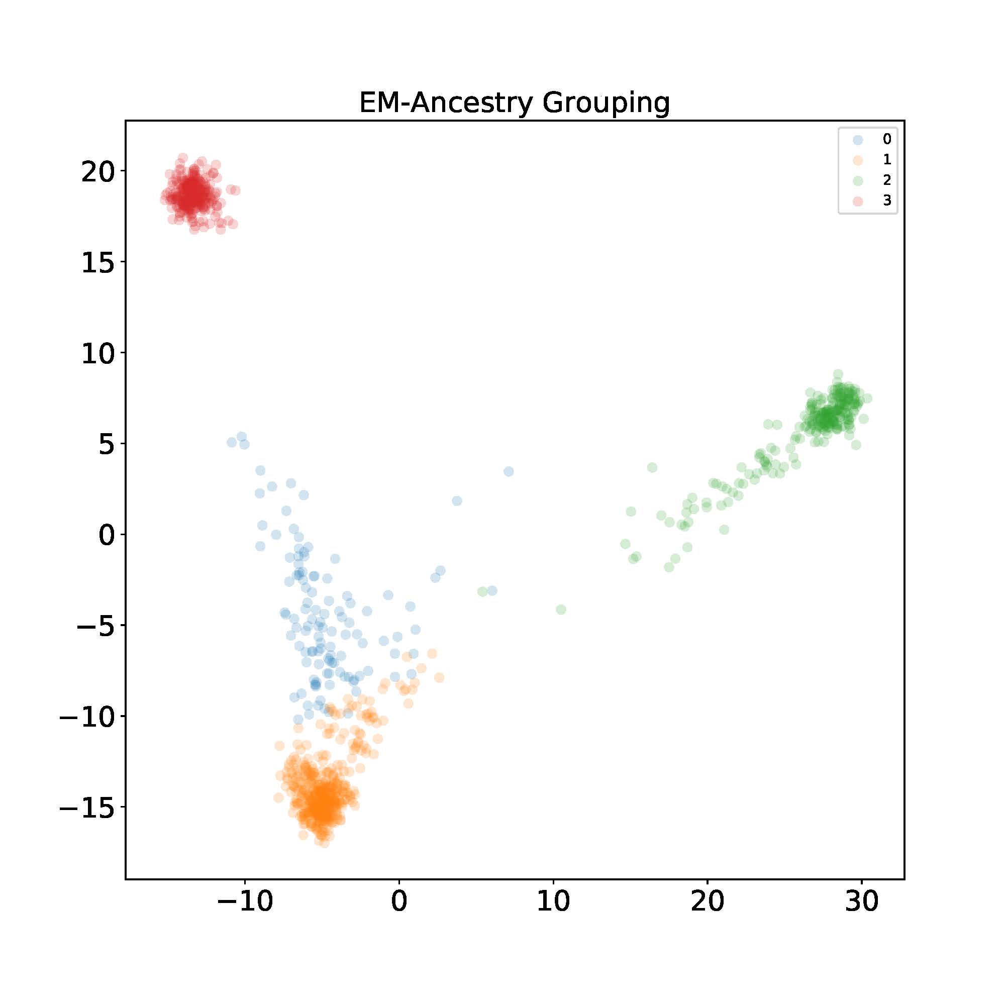
Let’s now implement the algorithm and see how it looks in the dataset described in the motivating example. After finishing running the EM algorithm, I label each individual with the index $k$ that gives the maximum probability for visualization purposes. Then I use PCA to project the data into 2D space. I found using $K=4$ ancestral components yields the best visual separation.
- Murphy, Kevin P. Machine learning: a probabilistic perspective. MIT press, 2012.
- Siva, Nayanah. “1000 Genomes project.” Nature biotechnology 26.3 (2008): 256-257.