Expectation-Maximization (EM) algorithm part II (EM-PCA)

In this section, we will explore another practical application of the EM-algorithm to speed up the computation of PCA. This section assumes the readers have already read my introduction part of EM algorithm.

Classical PCA

In classical PCA, given an input matrix $\mathbf{X} \in \mathbb{R}^{N \times M}$ (In genetic settings, $N$ can be the number of individuals, and $M$ be the number of SNPs), the goal is to find an orthonormal matrix $W \in \mathbb{R}^{m\times K}$ containing $K$ orthonormal vectors; and the corresponding scores (weight) along each vector $z \in \mathbb{R}^K$ , such that each individual $\mathbf{X}_i \in \mathbb{R}^m$ can be reconstructed using $\hat{\mathbf{x}}_i = \mathbf{Wz}_i$ with the minimum error. Mathematically, we are trying the minimize: \(\begin{align} J(\mathbf{W},\mathbf{Z}) = \frac{1}{N} || \mathbf{X} - \mathbf{ZW}^T ||_F^2 \end{align}\)

Under the constraint that $\mathbf{W}$ is an orthonormal matrix, the PC scores for each individual are therefore uncorrelated. Moreover, it can be proved by induction that the orthonormal matrix $\mathbf{W}$ is the eigenvectors corresponding to the top-$K$ largest eigenvalues, which implies it captures the top-$K$ variance when projecting X into the lower dimensional orthonormal subspace.

EM PCA

If we treat the dimensional reduction method as a probabilistic model, then the score matrix $\mathbf{Z}$ becomes a probabilistic distribution, and suppose we have the following assumptions:

• Underlying latent variable has a Gaussian distribution
• There is a linear relationship between latent and observed variables
• Isotropic Gaussian noise (covariance proportional to an identity matrix) in observed dimension

Then we can set up the model as

Notice here we can assume $\mathbf{\mu}_0 = \pmb{0}$ and $\mathbf{\Sigma} = \mathbf{I}$ without losing generality, since if they are not, we can always find another $\mathbf{W}’ = \mathbf{WU}$ such that $\mathbf{Uz} \sim \mathcal{N}(\pmb{0},\mathbf{I})$.

Then the marginal probability of $\mathbf{x}$ can be expressed as \(\begin{align} p(\mathbf{x}) = \mathcal{N}(\mathbf{\mu},\mathbf{WW}^T+\sigma^2\mathbf{I}) \end{align}\)

To see this, notice that \(\begin{align} \mathbb{E}[\mathbf{x}] = \mathbb{E}[\mathbf{\mu+Wz+\epsilon}] = \mathbf{\mu} + \mathbf{W}\mathbb{E}[\mathbf{z}] + \mathbb{E}[\mathbf{\epsilon}] = \mu \\ Var(\mathbb{x}) = \mathbb{E}[(\mathbf{\mu+Wz+\epsilon})(\mathbf{\mu+Wz+\epsilon})^T] = \mathbf{WW}^T + \sigma^2\mathbf{I} \end{align}\)

Further, the covariance can be easily calculated as \(\begin{align} Cov[\mathbf{x},\mathbf{z}] & = \mathbb{E}[(\mathbf{x}-\mathbf{\mu})(\mathbf{z}-\mathbf{0})^T] \\ &= \mathbb{E}[\mathbf{xz}^T - \mathbf{\mu z}^T] \\ &= \mathbb{E}[\mathbf{(Wz + \mu + \epsilon)z}^T] - \mathbf{\mu}\mathbb{E}[\mathbf{z}^T] \\ &= \mathbf{W}\mathbb{E}[\mathbf{zz}^T] \\ & = \mathbf{W} \end{align}\)

Then the joint probability is: \(p\left(\begin{bmatrix} \mathbf{z} \\ \mathbf{x} \end{bmatrix}\right) = \mathcal{N}\left(\begin{bmatrix} \mathbf{z} \\ \mathbf{x} \end{bmatrix} \bigg| \begin{bmatrix} \mathbf{0} \\ \boldsymbol{\mu} \end{bmatrix}, \begin{bmatrix} \mathbf{I} & \mathbf{W}^T \\ \mathbf{W} & \mathbf{WW}^T + \sigma^2\mathbf{I} \end{bmatrix}\right)\)

Applying Gaussian conditional probability, we get: \(p(\mathbf{z|x}) = \mathcal{N}(\mathbf{z | m, V}), \quad \mathbf{m} = \mathbf{W}^T(\mathbf{WW}^T + \sigma^2\mathbf{I})^{-1}(\mathbf{x} - \boldsymbol{\mu}), \quad \mathbf{V} = \mathbf{I} - \mathbf{W}^T(\mathbf{WW}^T + \sigma^2\mathbf{I})^{-1}\mathbf{W}\)

We can simplify the problem by standardizing our dataset $\pmb{X}$ so that $\pmb{\mu} = 0$. We, therefore, complete the setup of a typical EM algorithm.

In E-step, we compute \(% \begin{align} \lim_{\sigma \to 0}p(\mathbf{Z}|\mathbf{X}) = \mathbf{W}^T(\mathbf{WW}^T)^{-1}\mathbf{X}^T % \end{align}\) If $\sigma \neq 0$, the results would become probabilistic, in which case we don’t discuss. Notice that $\pmb{WW}^T$ is an $m \times m$ matrix, which takes $O(m^3)$ to compute the inverse. We instead cleverly apply the matrix inverse property to transform $\pmb{W}^T(\pmb{WW}^T)^{-1}$ to $(\pmb{W}^T\pmb{W})^{-1}\pmb{W}^T$, which reduces the inverse computation to $O(K^3)$, so that \(% \begin{align} \pmb{\hat{Z}} = (\pmb{W}^T\pmb{W})^{-1}\pmb{W}^T\pmb{X}^T % \end{align}\) In M-step, we compute the Q function \(\begin{align} & Q(\theta, \theta^{(t)}) = E[log(\pmb{X},\pmb{Z}| \pmb{W}, \sigma^2] \\ &= \sum_{i=1}^n p(\pmb{z}_i|\pmb{x}_i)(log(p(\pmb{x}_i|\pmb{z}_i)) + log(p(\pmb{z}_i))) \end{align}\) and by taking the partial derivative for $\pmb{W}$, we get \(% \begin{align} \pmb{\hat{W}} = \pmb{X}\pmb{Z}^T(\pmb{Z\pmb{Z}^T})^{-1} % \end{align}\) We thus complete the construction of the EM-PCA algorithm. Notice the complexity of the EM-PCA algorithm is dominated by $O(TKmn)$, and T is the number of iterations. This algorithm is linear regarding sample size and feature dimension, therefore bringing great advantage when the reduction dimension $K \ll m$ and $K \ll n$.

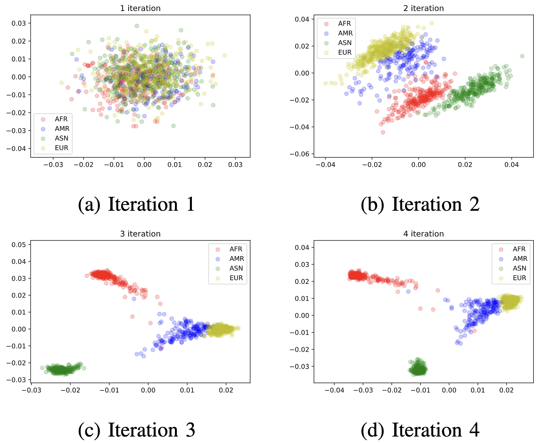
Experimental Results

Now let’s apply the algorithm to the 1000 Genome dataset to see how well the algorithm performs. As can be easily seen, EM-PCA has a fast convergence rate with a small runtime complexity.

References:

• Murphy, Kevin P. Machine learning: a probabilistic perspective. MIT press, 2012.
• Siva, Nayanah. “1000 Genomes project.” Nature biotechnology 26.3 (2008): 256-257.